43 how to add two data labels in excel pie chart
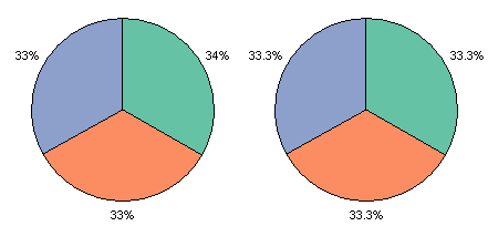
How to add two data labels for the same data on a pie chart? Consider using two sheets, a "Calculation" sheet and your "Dashboard" sheet. Create your pie graph as usual on the "Dashboard" sheet, but remove all labels. Adjust the colors as desired. On your "Calculation sheet, create the text for your percentage label and your ratio label. For example, the first pie chart charts the data 46 and 76. Custom data labels in a chart - Get Digital Help 21 Jan 2020 — Change the second series data source · Press with right mouse button on on the chart · Press with left mouse button on "Select Data" · Select the ...
Pie Chart in Excel - Inserting, Formatting, Filters, Data Labels Click on the Instagram slice of the pie chart to select the instagram. Go to format tab. (optional step) In the Current Selection group, choose data series "hours". This will select all the slices of pie chart. Click on Format Selection Button. As a result, the Format Data Point pane opens.
How to add two data labels in excel pie chart
Add data labels and callouts to charts in Excel 365 - EasyTweaks.com Step #1: After generating the chart in Excel, right-click anywhere within the chart and select Add labels . Note that you can also select the very handy option of Adding data Callouts. c# - Add data labels to excel pie chart - Stack Overflow I am drawing a pie chart with some data: private void DrawFractionChart(Excel.Worksheet activeSheet, Excel.ChartObjects xlCharts, Excel.Range xRange, Excel.Range yRange) { Excel.ChartObject ... Add data labels to excel pie chart. Ask Question Asked 9 years, 11 months ago. ... Is it legal for an airline to show, at the same exact time, two ... How to add data labels from different column in an Excel chart? Right click the data series in the chart, and select Add Data Labels > Add Data Labels from the context menu to add data labels. 2. Click any data label to select all data labels, and then click the specified data label to select it only in the chart. 3.
How to add two data labels in excel pie chart. Pie of Pie Chart in Excel - Inserting, Customizing, Formatting To add the data labels:- Select the chart and click on + icon at the top right corner of chart. Mark the check box containing data labels. Formatting Data Labels Consequently, this is going to insert default data labels on the chart. Edit titles or data labels in a chart - support.microsoft.com On a chart, click one time or two times on the data label that you want to link to a corresponding worksheet cell. The first click selects the data labels for the whole data series, and the second click selects the individual data label. Right-click the data label, and then click Format Data Label or Format Data Labels. Excel pie chart labels overlap arizona golden gloves. Search: R Pie Chart Labels Overlap.For example, x=[0,0 Click the Design tab in the Chart Tools section of the ribbon Instead of an overlapping window, graphics created in RStudio display inside the Plots pane A bar chart is a chart that visualizes data as a set of rectangular bars, their lengths being proportional to the values they represent To create a Bar of Pie chart ... Thread: Multiple data labels (in separate locations on chart) You can do it in a single chart. Create the chart so it has 2 columns of data. At first only the 1 column of data will be displayed. Move that series to the ...
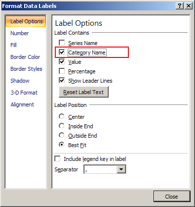
Adding data labels to a pie chart - OzGrid Free Excel/VBA Help Forum Re: Adding data labels to a pie chart. Thanks again, norie. Really appreciate the help. I tried recording a macro while doing it manually (before my first post). But it didn't record anything about labels, much less making them bold. Add or remove data labels in a chart - support.microsoft.com Click the data series or chart. To label one data point, after clicking the series, click that data point. In the upper right corner, next to the chart, click Add Chart Element > Data Labels. To change the location, click the arrow, and choose an option. If you want to show your data label inside a text bubble shape, click Data Callout. excel - Positioning data labels in pie chart - Stack Overflow Sub tester () Dim se As Series Set se = Totalt.ChartObjects ("Inosa gule").Chart.SeriesCollection ("Grøn pil") se.ApplyDataLabels With se.DataLabels .NumberFormat = "0,0 %" With .Format.Fill .ForeColor.RGB = RGB (255, 255, 255) .Transparency = 0.15 End With .Position = xlLabelPositionCenter End With End Sub Excel Pie Chart Labels on Slices: Add, Show & Modify Factors First of all, double-click on the data labels on the pie chart. As a result, a side window called Format Data Labels will appear. Then, go to the drop-down of the Label Options to Label Options tab. After that, check the Percentages option and uncheck all other options. You will get the percentages in the data labels.
How to Combine or Group Pie Charts in Microsoft Excel Click on the first chart and then hold the Ctrl key as you click on each of the other charts to select them all. Click Format > Group > Group. All pie charts are now combined as one figure. They will move and resize as one image. Choose Different Charts to View your Data How to create a pie chart in excel create a Pie of Pie or Bar of Pie chart, follow these steps: 1. Select the data range (in this example B5:C14 ). 2. On the Insert tab, in the Charts group, choose the Pie button: Pivot Chart Data Label Help Needed - Microsoft Community Open the Excel file with Pivot Chart and enabled with Data Labels> Click on the Labels displayed in the Chart> Right-click> Click Format Data Labels> Label Options> Number> In the Category, select the format as per your requirement. Here is the reference article: Change the format of data labels in a chart. How To Show Two Sets of Data on One Graph in Excel Below are steps you can use to help add two sets of data to a graph in Excel: 1. Enter data in the Excel spreadsheet you want on the graph. To create a graph with data on it in Excel, the data has to be represented in the spreadsheet. For multiple variables that you want to see plotted on the same graph, entering the values into different ...
Pie Chart Rounding in Excel - Peltier Tech
Add a DATA LABEL to ONE POINT on a chart in Excel All the data points will be highlighted. Click again on the single point that you want to add a data label to. Right-click and select ' Add data label '. This is the key step! Right-click again on the data point itself (not the label) and select ' Format data label '. You can now configure the label as required — select the content of ...
EXCEL Charts: Column, Bar, Pie and Line
How to Create Multi-Category Charts in Excel? - GeeksforGeeks Step 1: Insert the data into the cells in Excel. Now select all the data by dragging and then go to "Insert" and select "Insert Column or Bar Chart". A pop-down menu having 2-D and 3-D bars will occur and select "vertical bar" from it. Select the cell -> Insert -> Chart Groups -> 2-D Column.

Excel 3-D Pie Charts
How to Make a 2010 Excel Pie Chart with Labels Both Inside and Outside Harassment is any behavior intended to disturb or upset a person or group of people. Threats include any threat of suicide, violence, or harm to another.
Excel 3-D Pie charts - Microsoft Excel 2007
How to Create and Format a Pie Chart in Excel - Lifewire To add data labels to a pie chart: Select the plot area of the pie chart. Right-click the chart. Select Add Data Labels . Select Add Data Labels. In this example, the sales for each cookie is added to the slices of the pie chart. Change Colors
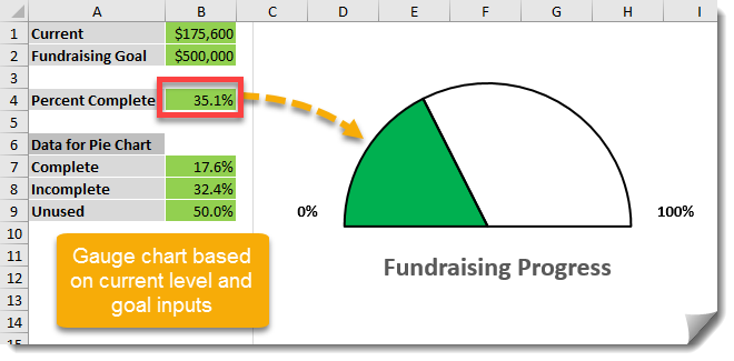
How To Create A Gauge Chart For Measuring Progress Against A Goal | How To Excel
How to Add Two Data Labels in Excel Chart (with Easy Steps) 7 Jul 2022 — Select any column representing demand units. Then right-click your mouse to bring the menu. After that, select Add Data Labels. Excel ...
Post a Comment for "43 how to add two data labels in excel pie chart"