43 adding chart labels in excel
chandoo.org › wp › change-data-labels-in-chartsHow to Change Excel Chart Data Labels to Custom Values? May 05, 2010 · The Chart I have created (type thin line with tick markers) WILL NOT display x axis labels associated with more than 150 rows of data. (Noting 150/4=~ 38 labels initially chart ok, out of 1050/4=~ 263 total months labels in column A.) It does chart all 1050 rows of data values in Y at all times. Excel Chart VBA - 33 Examples For Mastering Charts in Excel VBA Jun 17, 2022 · 30. Set Chart Data Labels and Legends using Excel VBA. You can set Chart Data Labels and Legends by using SetElement property in Excl VBA. Sub Ex_AddDataLabels() Dim cht As Chart 'Add new chart ActiveSheet.Shapes.AddChart.Select With ActiveChart 'Specify source data and orientation.SetSourceData Source:=Sheet1.Range("A1:B5"), …
Add data labels and callouts to charts in Excel 365 - EasyTweaks.com The steps that I will share in this guide apply to Excel 2021 / 2019 / 2016. Step #1: After generating the chart in Excel, right-click anywhere within the chart and select Add labels . Note that you can also select the very handy option of Adding data Callouts.
Adding chart labels in excel
Add or remove data labels in a chart - support.microsoft.com This displays the Chart Tools, adding the Design, and Format tabs. Do one of the following: ... Data labels make a chart easier to understand because they show details about a data series or its individual data points. ... You can add data labels to show the data point values from the Excel sheet in the chart. This step applies to Word for Mac ... How to Make a PIE Chart in Excel (Easy Step-by-Step Guide) Related tutorial: How to Copy Chart (Graph) Format in Excel Formatting the Data Labels. Adding the data labels to a Pie chart is super easy. Right-click on any of the slices and then click on Add Data Labels. As soon as you do this. data labels would be … TOP 9 what are data labels in excel BEST and NEWEST - Kiến Thức Về ... 7.Data Labels in Excel Pivot Chart (Detailed Analysis) - ExcelDemy. Author: . Post date: 10 yesterday. Rating: 5 (342 reviews) Highest rating: 5. Low rated: 2. Summary: Here, we change the appearances, and background, dynamic data label shows percentages/cell values as data labels in the Pivot chart in Excel.
Adding chart labels in excel. Add or remove data labels in a chart - support-uat.microsoft.com Do one of the following: On the Design tab, in the Chart Layouts group, click Add Chart Element, choose Data Labels, and then click None. Click a data label one time to select all data labels in a data series or two times to select just one data label that you want to delete, and then press DELETE. Right-click a data label, and then click Delete. Excel: How to Create a Bubble Chart with Labels - Statology To add labels to the bubble chart, click anywhere on the chart and then click the green plus "+" sign in the top right corner. Then click the arrow next to Data Labels and then click More Options in the dropdown menu: In the panel that appears on the right side of the screen, check the box next to Value From Cells within the Label Options ... How to Insert Axis Labels In An Excel Chart | Excelchat We have a sample chart as shown below; Figure 2 – Adding Excel axis labels. Next, we will click on the chart to turn on the Chart Design tab; We will go to Chart Design and select Add Chart Element; Figure 3 – How to label axes in Excel . In the drop-down menu, we will click on Axis Titles, and subsequently, select Primary Horizontal Figure ... › pie-chart-excelHow to Create a Pie Chart in Excel | Smartsheet Aug 27, 2018 · To create a pie chart in Excel 2016, add your data set to a worksheet and highlight it. Then click the Insert tab, and click the dropdown menu next to the image of a pie chart. Select the chart type you want to use and the chosen chart will appear on the worksheet with the data you selected.
How to Add Labels in Bubble Chart in Excel? - tutorialspoint.com Step 4. Add Labels − To add labels to the bubble chart, click anywhere on the chart and then click the "+" sign in the upper right corner. Then click the arrow beside Data Labels, followed by More Options in the drop-down menu. Step 5. In the panel that appears on the right side of the screen, check the box next to Value from Cells within the ... Add or remove data labels in a chart - support.microsoft.com Add data labels to a chart Click the data series or chart. To label one data point, after clicking the series, click that data point. In the upper right corner, next to the chart, click Add Chart Element > Data Labels. To change the location, click the arrow, and choose an option. How to Create a Pie Chart in Excel | Smartsheet Aug 27, 2018 · To create a pie chart in Excel 2016, add your data set to a worksheet and highlight it. Then click the Insert tab, and click the dropdown menu next to the image of a pie chart. Select the chart type you want to use and the chosen chart will appear on the worksheet with the data you selected. How to Change Axis Labels in Excel (3 Easy Methods) For changing the label of the vertical axis, follow the steps below: At first, right-click the category label and click Select Data. Then, click Edit from the Legend Entries (Series) icon. Now, the Edit Series pop-up window will appear. Change the Series name to the cell you want. After that, assign the Series value.
How to Change Excel Chart Data Labels to Custom Values? - Chandoo.org May 05, 2010 · The Chart I have created (type thin line with tick markers) WILL NOT display x axis labels associated with more than 150 rows of data. (Noting 150/4=~ 38 labels initially chart ok, out of 1050/4=~ 263 total months labels in column A.) It does chart all 1050 rows of data values in Y at all times. trumpexcel.com › pie-chartHow to Make a PIE Chart in Excel (Easy Step-by-Step Guide) Related tutorial: How to Copy Chart (Graph) Format in Excel Formatting the Data Labels. Adding the data labels to a Pie chart is super easy. Right-click on any of the slices and then click on Add Data Labels. As soon as you do this. data labels would be added to each slice of the Pie chart. Comparison Chart in Excel | Adding Multiple Series Under Same … This window helps you modify the chart as it allows you to add the series (Y-Values) as well as Category labels (X-Axis) to configure the chart as per your need. Under Legend Entries ( S eries) inside the Select Data Source window, you need to select the … › solutions › excel-chatHow to Insert Axis Labels In An Excel Chart | Excelchat We have a sample chart as shown below; Figure 2 – Adding Excel axis labels. Next, we will click on the chart to turn on the Chart Design tab; We will go to Chart Design and select Add Chart Element; Figure 3 – How to label axes in Excel . In the drop-down menu, we will click on Axis Titles, and subsequently, select Primary Horizontal Figure ...
Excel Custom Chart Labels • My Online Training Hub
› comparison-chart-in-excelComparison Chart in Excel | Adding Multiple Series Under Same ... This window helps you modify the chart as it allows you to add the series (Y-Values) as well as Category labels (X-Axis) to configure the chart as per your need. Under Legend Entries ( S eries) inside the Select Data Source window, you need to select the sales values for the year 2018 and year 2019.
Excel Chart Elements: Parts of Charts in Excel | ExcelDemy
Adding Colored Regions to Excel Charts - Duke Libraries Center … Nov 12, 2012 · Change the “years… in decline” series to an area chart; Select and adjust the x axis labels and ticks; Adjust the y axis range; Customize the color, label, and order of the data series; The basic mechanism of the colored regions on the chart is to use Excel’s “area chart” to create rectangular areas.

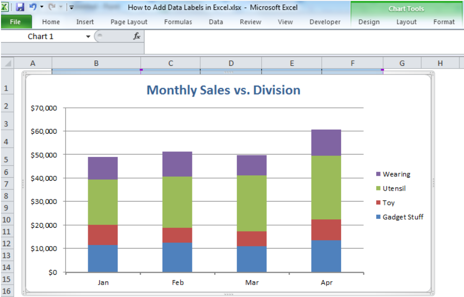
How to add total labels to stacked column chart in Excel?
How To Create Labels In Excel 18 Images - How To Print Labels From ... Here are a number of highest rated How To Create Labels In Excel pictures on internet. We identified it from honorable source. Its submitted by presidency in the best field. We allow this nice of How To Create Labels In Excel graphic could possibly be the most trending topic bearing in mind we part it in google plus or facebook.
Add a label and other information to axes in a Graph or Chart in Excel by Excel Made Easy
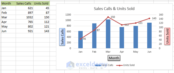
Multiple Series in One Excel Chart - Peltier Tech Aug 09, 2016 · Note: The default Excel chart has a legend, and I’ve replaced it with color-coded data labels on the last point of each series in the chart. ... This dialog differs from the one seen when adding data to an XY Scatter chart, because there is no place for X values (or X labels). To change the X labels, click the Edit button above the list of X ...

Lesson 2 | How to Create Charts Using Microsoft Excel Tutorial
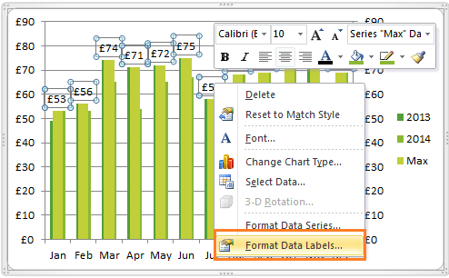
How to Add Text Labels in Excel Chart (4 Quick Methods) - ExcelDemy Steps: In the beginning, right-click on the data series of the chart. Next, select Add Data Labels and click Add Data Labels. Now, we can see in the screenshot below that all the data labels are added successfully to the chart. After that, right-click the data series and click Format Data Labels.
How to Add Data Labels in Excel - Excelchat | Excelchat
Add or remove data labels in a chart - support.microsoft.com Add data labels to a chart Click the data series or chart. To label one data point, after clicking the series, click that data point. In the upper right corner, next to the chart, click Add Chart Element > Data Labels. To change the location, click the arrow, and choose an option.

Excel Custom Chart Labels • My Online Training Hub
How to Make a Pie Chart in Excel & Add Rich Data Labels to The Chart! Creating and formatting the Pie Chart. 1) Select the data. 2) Go to Insert> Charts> click on the drop-down arrow next to Pie Chart and under 2-D Pie, select the Pie Chart, shown below. 3) Chang the chart title to Breakdown of Errors Made During the Match, by clicking on it and typing the new title.
Creating a chart with dynamic labels - Microsoft Excel 2013
How to add or move data labels in Excel chart? - ExtendOffice To add or move data labels in a chart, you can do as below steps: In Excel 2013 or 2016. 1. Click the chart to show the Chart Elements button . 2. Then click the Chart Elements, and check Data Labels, then you can click the arrow to choose an option about the data labels in the sub menu. See screenshot:

10 Design Tips to Create Beautiful Excel Charts and Graphs in 2017
Data Labels in Excel Pivot Chart (Detailed Analysis) Next open Format Data Labels by pressing the More options in the Data Labels. Then on the side panel, click on the Value From Cells. Next, in the dialog box, Select D5:D11, and click OK. Right after clicking OK, you will notice that there are percentage signs showing on top of the columns. 4. Changing Appearance of Pivot Chart Labels
How to create an Excel chart with no numerical labels? - Super User
analysistabs.com › excel-vba › chart-examples-tutorialsExcel Chart VBA - 33 Examples For Mastering Charts in Excel VBA Jun 17, 2022 · 30. Set Chart Data Labels and Legends using Excel VBA. You can set Chart Data Labels and Legends by using SetElement property in Excl VBA. Sub Ex_AddDataLabels() Dim cht As Chart 'Add new chart ActiveSheet.Shapes.AddChart.Select With ActiveChart 'Specify source data and orientation.SetSourceData Source:=Sheet1.Range("A1:B5"), PlotBy:=xlColumns ...
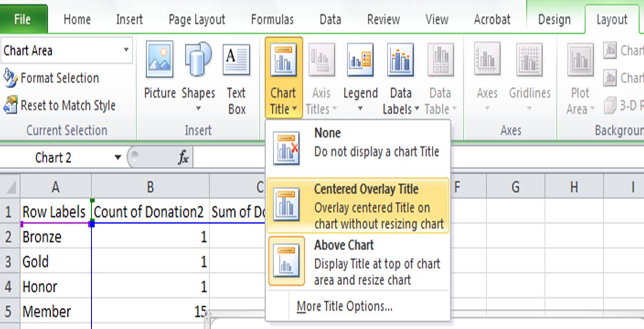
Excel Chart Options: Adding Titles | Pryor Learning Solutions
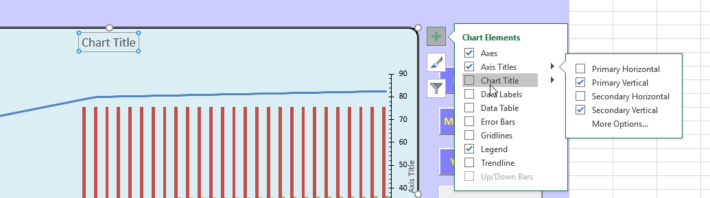
How to Add Axis Labels in Excel Charts - Step-by-Step (2022) - Spreadsheeto How to add axis titles 1. Left-click the Excel chart. 2. Click the plus button in the upper right corner of the chart. 3. Click Axis Titles to put a checkmark in the axis title checkbox. This will display axis titles. 4. Click the added axis title text box to write your axis label.

Charting in Excel - Adding Data Labels - YouTube
peltiertech.com › multiple-series-in-one-excel-chartMultiple Series in One Excel Chart - Peltier Tech Aug 09, 2016 · This dialog differs from the one seen when adding data to an XY Scatter chart, because there is no place for X values (or X labels). To change the X labels, click the Edit button above the list of X labels in the chart. The Axis Labels dialog appears.
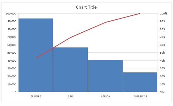
Create a Pareto Chart With Excel 2016 | Free Microsoft Excel Tutorials
How to Add X and Y Axis Labels in Excel (2 Easy Methods) In short: Select graph > Chart Design > Add Chart Element > Axis Titles > Primary Horizontal. Afterward, if you have followed all steps properly, then the Axis Title option will come under the horizontal line. But to reflect the table data and set the label properly, we have to link the graph with the table.
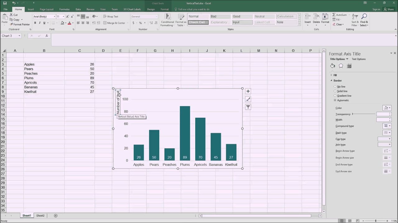
Adding horizontally-aligned y-axis titles to charts in Excel 2016 - YouTube
Excel charts: add title, customize chart axis, legend and data labels Click the Chart Elements button, and select the Data Labels option. For example, this is how we can add labels to one of the data series in our Excel chart: For specific chart types, such as pie chart, you can also choose the labels location. For this, click the arrow next to Data Labels, and choose the option you want.

32 Excel Chart Add Label - Labels Design Ideas 2020
Text Labels on a Horizontal Bar Chart in Excel - Peltier Tech Dec 21, 2010 · In Excel 2003 the chart has a Ratings labels at the top of the chart, because it has secondary horizontal axis. Excel 2007 has no Ratings labels or secondary horizontal axis, so we have to add the axis by hand. On the Excel 2007 Chart Tools > Layout tab, click Axes, then Secondary Horizontal Axis, then Show Left to Right Axis.

Excel Solution - How to Create Custom Data Label in Chart.avi - YouTube
How to add data labels in excel to graph or chart (Step-by-Step) Add data labels to a chart. 1. Select a data series or a graph. After picking the series, click the data point you want to label. 2. Click Add Chart Element Chart Elements button > Data Labels in the upper right corner, close to the chart. 3. Click the arrow and select an option to modify the location. 4.
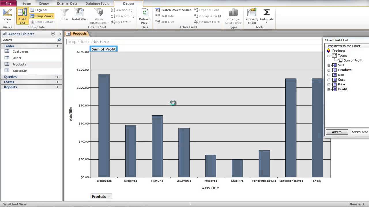
How to Create a Pivot Chart in Microsoft Access - YouTube
How to Add Data Labels in Excel - Excelchat | Excelchat After inserting a chart in Excel 2010 and earlier versions we need to do the followings to add data labels to the chart; Click inside the chart area to display the Chart Tools. Figure 2. Chart Tools Click on Layout tab of the Chart Tools. In Labels group, click on Data Labels and select the position to add labels to the chart. Figure 3.
Post a Comment for "43 adding chart labels in excel"