38 conditional formatting pivot table row labels
Pivot Table Grouping, Ungrouping And Conditional Formatting So let's drag the Age under the Rows area to create our Pivot table. #1) Right-click on any number in the pivot table. #2) On the context menu, click Group. #3) Grouping dialog box appears, in this example, the least number is 25, so by default the Starting number is entered as 25, and you can change if necessary. Pivot table conditional formatting based on row label trabalhos Busque trabalhos relacionados a Pivot table conditional formatting based on row label ou contrate no maior mercado de freelancers do mundo com mais de 21 de trabalhos. Cadastre-se e oferte em trabalhos gratuitamente.
Excel VBA: Conditional Format of Pivot Table based on Column Label myPivotSourceName = myPivotField.Name. Then rather than referencing the data field with the pivot field object, I referenced the DataRange with the string: myPivotTable.PivotFields (myPivotSourceName).DataRange.Select. Works perfectly and is completely portable for any pivottable on any sheet with any fields. excel vba.
Conditional formatting pivot table row labels
Design the layout and format of a PivotTable Right-click the field name and then select the appropriate command — Add to Report Filter, Add to Column Label, Add to Row Label, or Add to Values — to place the field in a specific area of the layout section. Click and hold a field name, and then drag the field between the field section and an area in the layout section. Conditional Formatting on Pivot Table row labels In srcFromPowerPivot sheet cell A is from powerpivot under row label comparing the dates in cell C (3 dates) and the condtional formatting doesnt work. In cell J it worked cos I dragged under value instead of row label. In the srcFromWorksheet it worked even though it is under rowlabel. Sheet3 is just a copy of powerpivot data. Conditional formatting for Pivot Tables in Excel 2016 - 2007 Conditional formatting when applied to PivotTables in Excel 2007 - 2016 is applied to the underlying structure of the PivotTable rather than to the cells themselves. So, when you interact with a PivotTable such as moving fields around and viewing your data in different ways, the formatting is updated as you work.
Conditional formatting pivot table row labels. Pivot Table Conditional Formatting with VBA - Peltier Tech A reader encountered problems applying conditional formatting to a pivot table. I tried it myself, using the same kind of formulas I would have applied in a regular worksheet range, and had no problem. ... including what I think you meant with your last suggestions (and Text1 is one of my Row Labels, and Text is one of the names populating ... How to Apply Conditional Formatting to Pivot Tables So in this post I explain how to apply conditional formatting for pivot tables. 1. Select a cell in the Values area The first step is to select a cell in the Values area of the pivot table. If your pivot table has multiple fields in the Values area, select a cell for the field you want to apply the formatting to. 2. Apply Conditional Formatting Overwrite pivot table conditional format based on row label As far as I know, using the one rule in the Conditional formatting, we can only format the cells with one color if the condition is true and if the same condition is false, the formatting of the cell will be blank and if both conditions are true, the formatting of cell depends on the highest ranking/priority of the rules in Conditional formatting. Excel Pivot Table Conditional Formatting Row Labels Go making the conditional formatting select the color scale and do it based on commercial and choose diverging and the colors should give expected result. Here a glaze color or bar and been applied...
Conditional Formatting in Pivot Table (Example) - EDUCBA Click on any cell in the pivot table > Go to the HOME tab > Click on Conditional Formatting option under Styles option > Click on Manage Rules option. It will open a Rules Manager dialog box. Click on the Edit Rule tab, as shown in the below screenshot. It will open the Editing Rule formatting window. Refer to the below screenshot. EOF Re-Apply Pivot Table Conditional Formatting - yoursumbuddy This method relies on all the conditional formatting you want to re-apply being in that first row labels cell. In cases where the conditional formatting might not apply to the leftmost row label, I've still applied it to that column, but modified the condition to check which column it's in. This function can be modified and called from a ... Format Pivot Table Labels Based on Date Range In the pivot table, remove any filters that have been applied - all the rows need to be visible before you apply the conditional formatting. Select all the dates in the Row Labels that you want to format. On the Ribbon, click the Home tab, and then in the Styles group, click Conditional Formatting.
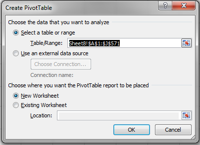
Conditional Formatting in Pivot Table - WallStreetMojo We must follow the steps to apply conditional formatting in the pivot table. First, we must select the data. Then, in the "Insert" Tab, click on "Pivot Tables." As a result, a dialog box appears. Next, we must insert the pivot table in a new worksheet by clicking "OK." Currently, a pivot table is blank. Next, we need to bring in the values. Conditional Format Pivot Table Row - Chandoo.org Select the entire row, and when you apply the conditional format, make the column reference absolute. So, say we want the entire row 2 to be formatted if cell in col B = 5. formula would be: =$B2=5 Pivot table conditional formatting - Exceljet Select any cell in the data you wish to format and then choose "New rule" from the conditional formatting menu on the Home tab of the ribbon. At the top of the window, you will see setting for which cells to apply conditional formatting to. For the example shown, we want: "All cells showing sum of "sales values" for name and "date" Conditional formatting for Pivot Tables in Excel 2016 - 2007 Conditional formatting when applied to PivotTables in Excel 2007 - 2016 is applied to the underlying structure of the PivotTable rather than to the cells themselves. So, when you interact with a PivotTable such as moving fields around and viewing your data in different ways, the formatting is updated as you work.
Sorting a Pivot Table | MyExcelOnline
Conditional Formatting on Pivot Table row labels In srcFromPowerPivot sheet cell A is from powerpivot under row label comparing the dates in cell C (3 dates) and the condtional formatting doesnt work. In cell J it worked cos I dragged under value instead of row label. In the srcFromWorksheet it worked even though it is under rowlabel. Sheet3 is just a copy of powerpivot data.

Create Beautiful Reports with Custom Pivot Tables and JavaScript Spreadsheets | SpreadJS
Design the layout and format of a PivotTable Right-click the field name and then select the appropriate command — Add to Report Filter, Add to Column Label, Add to Row Label, or Add to Values — to place the field in a specific area of the layout section. Click and hold a field name, and then drag the field between the field section and an area in the layout section.

dynamic - Conditional Formatting Pivot table in Google Sheets - Stack Overflow
Finding Duplicates by Using Conditional Formatting in Excel 2010

34 Using The Current Worksheets Pivot Table Add The Task Name As A Column Label - Labels ...

Using column label as formatting condition in excel pivot table - Stack Overflow

Finding Duplicates by Using Conditional Formatting in Excel 2010

How To Find And Remove Duplicates In A Pivot Table - MS Excel | Excel In Excel

85 DOWNLOAD PRINTABLE HOW DO I PIVOT TABLE IN EXCEL PDF DOC ZIP - Pivot

33 Pivot Table Blank Row Label - Labels Database 2020

How to Apply Conditional Formatting in Pivot Table? (with Example)
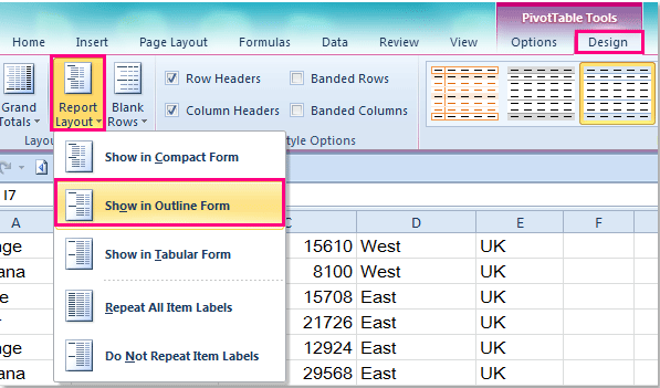
How to repeat row labels for group in pivot table?

Learn How to Apply Conditional Formatting in a Pivot Table | Excelchat
Pivoting-tour
Conditional Formatting of Row in Text Table based on Dimension

pivot table - Conditional formatting between 2 sheets - Super User
Post a Comment for "38 conditional formatting pivot table row labels"