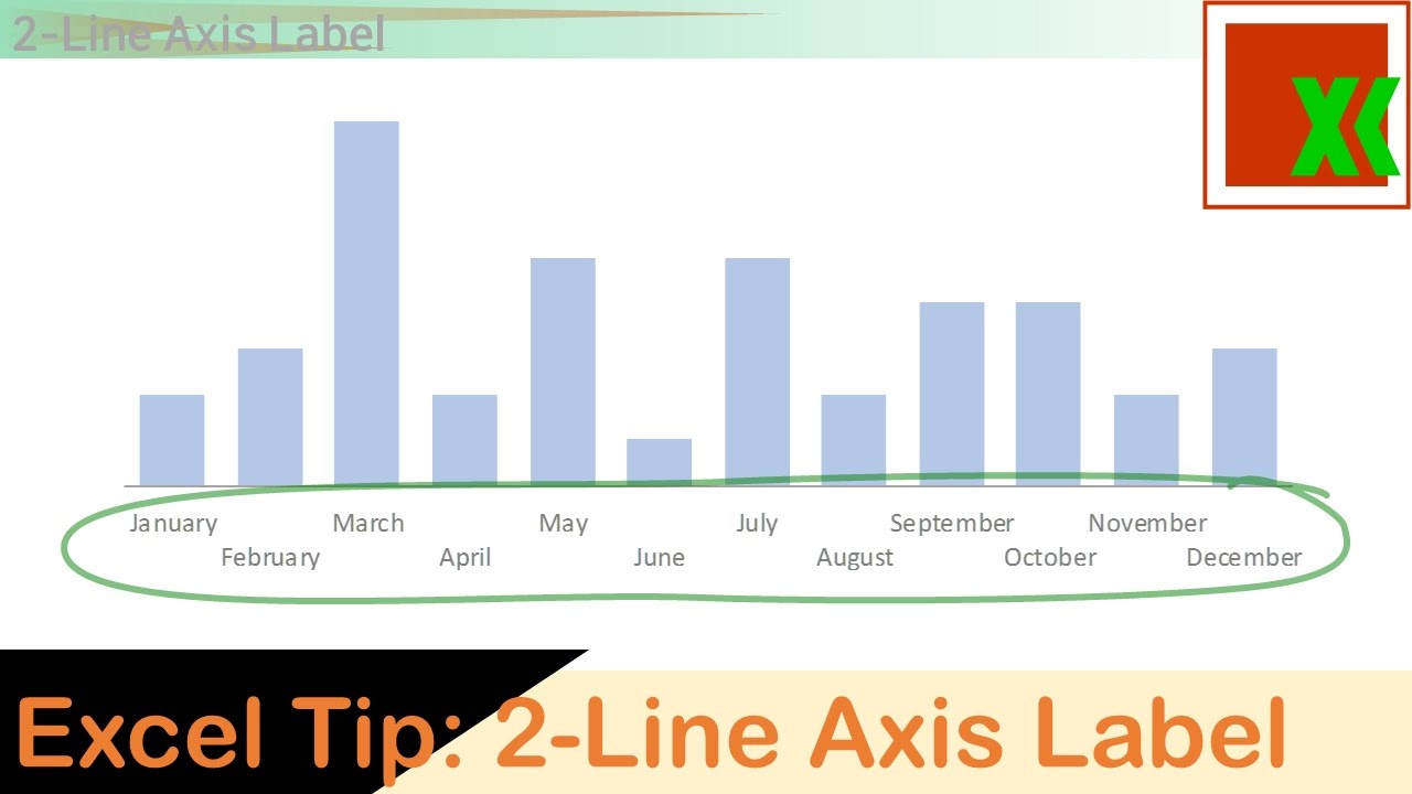
44 how to add data labels to a pie chart in excel on mac

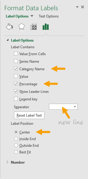
Office: Display Data Labels in a Pie Chart 2. If you have not inserted a chart yet, go to the Insert tab on the ribbon, and click the Chart option. 3. In the Chart window, choose the Pie chart option from the list on the left. Next, choose the type of pie chart you want on the right side. 4. Once the chart is inserted into the document, you will notice that there are no data labels. How to display leader lines in pie chart in Excel? To display leader lines in pie chart, you just need to check an option then drag the labels out. 1. Click at the chart, and right click to select Format Data Labels from context menu. 2. In the popping Format Data Labels dialog/pane, check Show Leader Lines in the Label Options section. See screenshot: 3.

How to Create and Format a Pie Chart in Excel - Lifewire To add data labels to a pie chart: Select the plot area of the pie chart. Right-click the chart. Select Add Data Labels . Select Add Data Labels. In this example, the sales for each cookie is added to the slices of the pie chart. Change Colors

How to add data labels to a pie chart in excel on mac

Microsoft Excel Tutorials: Add Data Labels to a Pie Chart To add the numbers from our E column (the viewing figures), left click on the pie chart itself to select it: The chart is selected when you can see all those blue circles surrounding it. Now right click the chart. You should get the following menu: From the menu, select Add Data Labels. New data labels will then appear on your chart: How to show percentage in pie chart in Excel? Select the data you will create a pie chart based on, click Insert > I nsert Pie or Doughnut Chart > Pie. See screenshot: 2. Then a pie chart is created. Right click the pie chart and select Add Data Labels from the context menu. 3. Now the corresponding values are displayed in the pie slices. How to Create Pie Charts in Excel (In Easy Steps) Select the pie chart. 9. Click the + button on the right side of the chart and click the check box next to Data Labels. 10. Click the paintbrush icon on the right side of the chart and change the color scheme of the pie chart. Result: 11. Right click the pie chart and click Format Data Labels. 12.

How to add data labels to a pie chart in excel on mac. Add or remove data labels in a chart - support.microsoft.com Click the data series or chart. To label one data point, after clicking the series, click that data point. In the upper right corner, next to the chart, click Add Chart Element > Data Labels. To change the location, click the arrow, and choose an option. If you want to show your data label inside a text bubble shape, click Data Callout. Create a chart in Excel for Mac Click a specific chart type and select the style you want. With the chart selected, click the Chart Design tab to do any of the following: Click Add Chart Element to modify details like the title, labels, and the legend. Click Quick Layout to choose from predefined sets of chart elements. Pie charts - Google Docs Editors Help Double-click the chart you want to change. At the right, click Customize. Choose an option: Chart style: Change how the chart looks. Pie chart: Add a slice label, doughnut hole, or change border color. Chart & axis titles: Edit or format title text. Pie slice: Change color of the pie slice, or pull out a slice from the center. Add or remove data labels in a chart - support.microsoft.com On the Design tab, in the Chart Layouts group, click Add Chart Element, choose Data Labels, and then click None. Click a data label one time to select all data labels in a data series or two times to select just one data label that you want to delete, and then press DELETE. Right-click a data label, and then click Delete.

Pie Chart in Excel | How to Create Pie Chart | Step-by ... Step 1: Do not select the data; rather, place a cursor outside the data and insert one PIE CHART. Go to the Insert tab and click on a PIE. Step 2: once you click on a 2-D Pie chart, it will insert the blank chart as shown in the below image. Step 3: Right-click on the chart and choose Select Data. How to Make a Pie Chart in Excel: 10 Steps (with Pictures) If you would rather make a chart from data you already have, double-click the Excel document that contains the data to open it and proceed to the next section. 2 Click Blank workbook (PC) or Excel Workbook (Mac). It's in the top-left side of the "Template" window. 3 Add a name to the chart. How Do You Add Text To Pie Chart In Excel For Mac - needtree To add data labels to a pie chart: How Do You Add Text To Pie Chart In Excel For Mac Free. Select the plot area of the pie chart. Right-click the chart. Select Add Data Labels. In this example, the sales for each cookie is added to the slices of the pie chart. How to format the data labels in Excel:Mac 2011 when ... Try clicking on Column or Row you want to set. Go to Format Menu Click cells Click on Currency Change number of places to 0 (zero) (if in accounting do the same thing. _________ Disclaimer: The questions, discussions, opinions, replies & answers I create, are solely mine and mine alone, and do not reflect upon my position as a Community Moderator.

How to Use Cell Values for Excel Chart Labels Select the chart, choose the "Chart Elements" option, click the "Data Labels" arrow, and then "More Options.". Uncheck the "Value" box and check the "Value From Cells" box. Select cells C2:C6 to use for the data label range and then click the "OK" button. The values from these cells are now used for the chart data labels. How to Create a Pie Chart from a Single Column [FREE ... Navigate to the Insert tab. Hit the " Insert Pie or Doughnut Chart " button. Under " 2-D Pie, " click " Pie. ". Once you do that, Excel will automatically plot a pie graph using your pivot table. Step 3. Clean up Your Pie Chart. Before calling it a day, let's remove the field buttons related to our pivot table to make the graph ... How to Make a Pie Chart in Microsoft Excel Go to the Insert tab and click the Pie Chart drop-down arrow. In Excel on the web, this is simply a button because there is currently only one pie chart design available. On Windows or Mac, select ... How to Create a Pie Chart in Excel - Smartsheet If want the category names to appear on or near the chart, right-click on the chart and click Add Data Labels …. By default, the numerical values are added. To add other labels, such as the categorical values or the percentage of the total that each category represents, right-click on the chart, then click Format Data Labels ….

[最も人気のある！] excel chart series name from cell 122385-Excel chart series name from cell ...

Excel charts: add title, customize chart axis, legend and ... To add a label to one data point, click that data point after selecting the series. Click the Chart Elements button, and select the Data Labels option. For example, this is how we can add labels to one of the data series in our Excel chart: For specific chart types, such as pie chart, you can also choose the labels location.

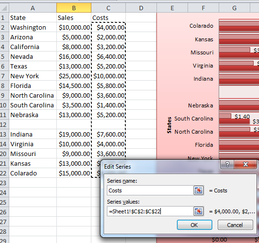
【ベストコレクション】 change series name excel 285790-How to change series name in excel ipad

How to Make a Pie Chart in Excel. Part of a new series of ... While holding control+alt, click and drag to select the data representing the second variable, just as you did in the previous step. In our case, it's "Measure 2". The result should look something like this: You have now selected the data you will use to make a pie chart. Next step is to make the pie chart using the data selected.

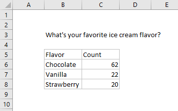
Pie Chart: Survey results favorite ice cream flavor | Exceljet

How to Insert Pie Chart in WPS Spreadsheet | WPS Academy ... We select Pie here to insert a pie chart in the table. Select the pie chart, click the Chart Element button at the top right of the chart, check the Data Labels icon and then the pie chart shows the values. Then click the triangle icon on the right of Data Labels, select Outside End, and the values are show n outside the chart. The data label ...

30 Label X And Y Axis In Excel - Best Labeling Ideas

How do I create a pie chart in Excel ... How do you make a pie chart on Microsoft Excel? Enter and Select the Tutorial Data. A pie chart is a visual representation of data and is used to display the amounts of several categories relative to the total value ; Create the Basic Pie Chart. Add the Chart Title. Add Data Labels to the Pie Chart. Change Colors. Explode a Piece of the Pie Chart.

31 How To Label Chart Axis In Excel - Labels For Your Ideas

Excel 3-D Pie charts - Microsoft Excel 2016 - OfficeToolTips If you want to create a pie chart that shows your company (in this example - Company A) in the greatest positive light: Do the following: 1. Select the data range (in this example, B5:C10 ). 2. On the Insert tab, in the Charts group, choose the Pie button: Choose 3-D Pie. 3. Right-click in the chart area, then select Add Data Labels and click ...

Pie Chart: Survey results favorite ice cream flavor | Exceljet

How to add percentage to pie chart in excel - kasapwestcoast To add data labels, select the chart and then click on the + button in the top right corner of the pie chart and check the Data Labels button. Initially, the pie chart will not have any data labels in it. Select -> Insert -> Doughnut or Pie Chart -> 2-D Pie. Open Microsoft Excel and select the data that you want to create a pie.

Excel Vba Chart Title Centered Overlay - excel how can i neatly overlay a line graph series over ...

How to Make a PIE Chart in Excel (Easy Step-by-Step Guide) Related tutorial: How to Copy Chart (Graph) Format in Excel Formatting the Data Labels. Adding the data labels to a Pie chart is super easy. Right-click on any of the slices and then click on Add Data Labels. As soon as you do this. data labels would be added to each slice of the Pie chart.

When to Use Bar of Pie Chart in Excel 365? - Easy Tricks!!

How to show data label in "percentage" instead of ... Select Format Data Labels. Select Number in the left column. Select Percentage in the popup options. In the Format code field set the number of decimal places required and click Add. (Or if the table data in in percentage format then you can select Link to source.) Click OK. Regards, OssieMac. Report abuse.

Share :