42 excel pivot table 2 row labels
How to Create Excel Pivot Table [Includes practice file] 15.01.2022 · The area to the left results from your selections from [1] and [2]. You’ll see that the only difference I made in the last pivot table was to drag the AGE GROUP field underneath the PRECINCT field in the Row Labels quadrant. How to Create Excel Pivot Table. There are several ways to build a pivot table. Pivot Table "Row Labels" Header Frustration - Microsoft ... Hi Everyone please help I can't change my headers from Row Labels in a Pivot Table. Using Excel 365
Pivot Table Sort by second row label - Microsoft Community Ramz Aftab Replied on May 17, 2014 Here is how you can get the results: Place your cursor on Col. B data wherever Names are. Goto Home ribbon>Editing>Sort it in either way. Alternatively, you can Sort from Pivots settings. Ramz Aftab [ MOS 77-888/82 Excel Expert ] ramzaftab [at]gmail [.]com Report abuse Was this reply helpful?
Excel pivot table 2 row labels
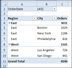
Repeat item labels in a PivotTable Right-click the row or column label you want to repeat, and click Field Settings. Click the Layout & Print tab, and check the Repeat item labels box. Make sure Show item labels in tabular form is selected. Notes: When you edit any of the repeated labels, the changes you make are applied to all other cells with the same label. How to reverse a pivot table in Excel? To reverse the pivot table, you need to open PivotTable and PivotChart Wizard dialog first and create a new pivot table in Excel. 1. Press Alt + D + P shortcut keys to open PivotTable and PivotChart Wizard dialog, then, check Multiple consolidation ranges option under Where is the data that you want to analyze section and PivotTable option under What kind of report do you … How to make row labels on same line in pivot table? Make row labels on same line with setting the layout form in pivot table As we all know, the pivot table has several layout form, the tabular form may help us to put the row labels next to each other. Please do as follows: 1. Click any cell in your pivot table, and the PivotTable Tools tab will be displayed. 2.
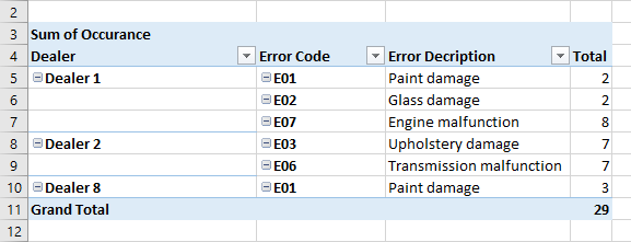
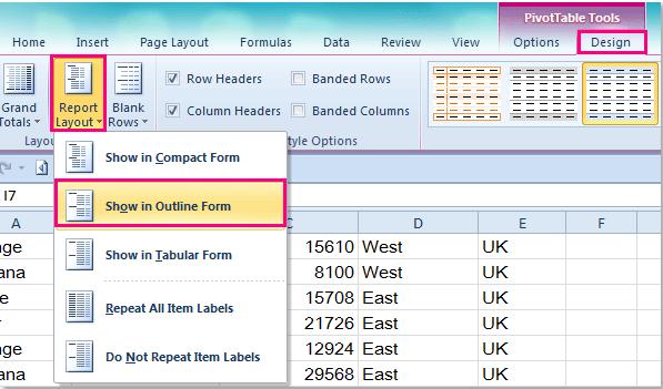
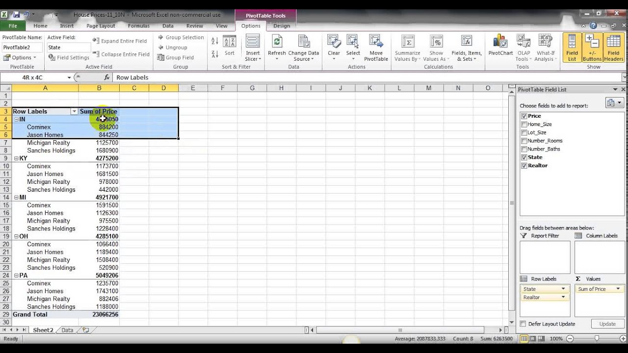
Excel pivot table 2 row labels. How to repeat row labels for group in pivot table? In Excel, when you create a pivot table, the row labels are displayed as a compact layout, all the headings are listed in one column. Sometimes, you need to convert the compact layout to outline form to make the table more clearly. But in tphe outline layout, the headings will be displayed at the top of the group. Pivot Table Row Labels In the Same Line - Beat Excel! First make a pivot table with required fields. Arrange the fields as shown in left picture. Your initial table will look like right picture. Now click on "Error Code" and access field settings. First check "None" option in "Subtotals & Filters" tab to disable totals after every row. How to rename group or row labels in Excel PivotTable? 1. Click at the PivotTable, then click Analyze tab and go to the Active Field textbox. 2. Now in the Active Field textbox, the active field name is displayed, you can change it in the textbox. You can change other Row Labels name by clicking the relative fields in the PivotTable, then rename it in the Active Field textbox. Pivot Table Two Row Labels Excel Pivot table row labels side by side - Excel Tutorials. Excel Details: Pivot table row labels side by side Posted on October 29, 2018 July 20, 2020 by Tomasz Decker If you use pivot tables there is a big chance that you want to place data labels side by side in different columns, instead of different rows. add row label pivot table › Verified 4 days ago
How to Create a Pivot Table in Excel: A Step-by-Step Tutorial 31.12.2021 · Your next step is to drag and drop a field — labeled according to the names of the columns in your spreadsheet — into the Row Labels area. This will determine what unique identifier — blog post title, product name, and so on — the pivot table will organize your data by. Remove PivotTable Duplicate Row Labels [SOLVED] Re: Remove PivotTable Duplicate Row Labels. Sometimes when the cells are stored in different formats within the same column in the raw data, they get duplicated. Also, if there is space/s at the beginning or at the end of these fields, when you filter them out they look the same, however, when you plot a Pivot Table, they appear as separate ... How to Customize Your Excel Pivot Chart Data Labels - dummies The Data Labels command on the Design tab's Add Chart Element menu in Excel allows you to label data markers with values from your pivot table. When you click the command button, Excel displays a menu with commands corresponding to locations for the data labels: None, Center, Left, Right, Above, and Below. None signifies that no data labels should be added to the chart and Show signifies ... Pivot table row labels side by side - Excel Tutorials You can copy the following table and paste it into your worksheet as Match Destination Formatting. Now, let's create a pivot table ( Insert >> Tables >> Pivot Table) and check all the values in Pivot Table Fields. Fields should look like this. Right-click inside a pivot table and choose PivotTable Options…. Check data as shown on the image below.
How to make row labels on same line in pivot table? Make row labels on same line with PivotTable Options. You can also go to the PivotTable Options dialog box to set an option to finish this operation.. 1.Click any one cell in the pivot table, and right click to choose PivotTable Options, see screenshot:. 2. How to Use Excel Pivot Table Label Filters The item is immediately hidden in the pivot table. Quickly Hide All But a Few Items. You can use a similar technique to hide most of the items in the Row Labels or Column Labels. Select the pivot table items that you want to keep visible; Right-click on one of the selected items; In the pop-up menu, click Filter, then click Keep Only Selected ... How to add side by side rows in excel pivot table ? | AnswerTabs You have to right-click on pivot table and choose the PivotTable options. Then swich to Display tab and turn on Classic PivotTable layout: Now the pivot table should look like this: As a next step, you have to modify the Field settings of the rows: In subtotals section choose None: The pivot table rows should be now placed next to each other: Excel Pivot Table Row labels - Stack Overflow Excel Pivot Table Row labels. Ask Question Asked 6 years, 4 months ago. Modified 6 years, 4 months ago. Viewed 366 times -1 I made a pivot table in Excel with three categories in the Rows box. I then copy-pasted the table into a new document. I want to have each row include the variables which I used in to create the pivot table.
Pivot table row labels side by side
Duplicate Items Appear in Pivot Table - Excel Pivot Tables Follow these steps to add a new field: Insert a new column in the source data, with the heading CityName. In Row 2 of the new column, enter the formula =TRIM (C2). Copy the formula down to the last row of data in the source table. If the source data is stored in an Excel Table, the formula should copy down automatically. Refresh the pivot table
Discover Pivot Tables – Excel’s most powerful feature and also least known
How to Insert a Blank Row in Excel Pivot Table | MyExcelOnline 17.01.2021 · Pivot Table reports are shown in a Compact Layout format as a default and if you have two or more Items in the Row Labels (e.g.Month & Customer), then the Pivot Table report can look very clunky…. There is a cool little trick that most Excel users do not know about that adds a blank row after each item, making the Pivot Table report look more appealing.

Design your Pivot Table in Excel | Excel in Excel
Pivot table - Wikipedia Row labels are used to apply a filter to one or more rows that have to be shown in the pivot table. For instance, if the "Salesperson" field is dragged on this area then the other output table constructed will have values from the column "Salesperson", i.e. , one will have a number of rows equal to the number of "Sales Person".
How to repeat row labels for group in pivot table?
pivot table how to combine 2 row labels | MrExcel Message ... pivot table how to combine 2 row labels sdsurzh Nov 6, 2013 S sdsurzh Board Regular Joined Sep 27, 2009 Messages 248 Nov 6, 2013 #1 Hi, i am having the pivot table in the below format. my concern is how i can combine both A & AA together the source is from data connection and not from the excel.

How To Create Pivot Table With Multiple Columns In Excel 2010 | Awesome Home
Excel Pivot Table Report - Clear All, Remove Filters, Select … Pivot Table Options tab - Actions group Customizing a Pivot Table report: When you insert a Pivot Table, a blank Pivot Table report is created in the specified location, and the 'PivotTable Field List' Pane also appears which allows you to Add or Remove Fields, Move Fields to different Areas and to set Field Settings. The 'Options' and 'Design' tabs (under the 'PivotTable Tools' …
33 Pivot Table Blank Row Label - Labels Database 2020
Automatic Row And Column Pivot Table Labels - How To Excel ... Select the data set you want to use for your table The first thing to do is put your cursor somewhere in your data list Select the Insert Tab Hit Pivot Table icon Next select Pivot Table option Select a table or range option Select to put your Table on a New Worksheet or on the current one, for this tutorial select the first option Click Ok

How to count unique values in pivot table?
How do I make multiple row labels in a pivot table? - idswater ... 3 Feb 2021 — How do I make multiple row labels in a pivot table? · Under the PivotTable Tools tab, click Design > Report Layout > Show in Tabular Form, see ...
Repeat Pivot Table Labels in Excel 2010 – Excel Pivot Tables
Excel Pivot Table Group: Step-By-Step Tutorial To Easily Group … Let's start by looking at the… Example Pivot Table And Source Data. This Pivot Tutorial is accompanied by an Excel workbook example. If you want to follow each step of the way and see the results of the processes I explain below, you can get immediate free access to this workbook by subscribing to the Power Spreadsheets Newsletter.. I use the following source data for all …

How to Sort Pivot Table Row Labels, Column Field Labels and Data Values with Excel VBA Macro ...
How to group time by hour in an Excel pivot table? Now the pivot table is added. Right-click any time in the Row Labels column, and select Group in the context menu. See screenshot: 5. In the Grouping dialog box, please click to highlight Hours only in the By list box, and click the OK button. See screenshot: Now the time data is grouped by hours in the newly created pivot table. See screenshot:
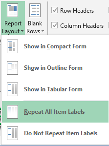
Repeat All Item Labels In An Excel Pivot Table | MyExcelOnline
Excel Pivot Table Report Layout - Contextures Excel Tips 15.01.2022 · Pivot Table Layout. In Excel, Pivot tables have a defined basic structure, called a Pivot Table Report Layout, or Pivot Table Form. On this page, you'll find information about the 3 types of pivot table report layouts: - Compact, Outline, Tabular. With the following details about each report layout type: report layout examples; features and ...
33 Pivot Table Blank Row Label - Labels Database 2020
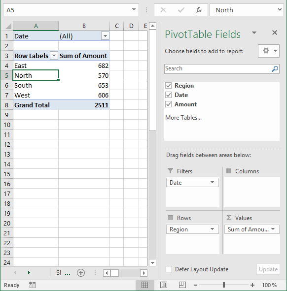
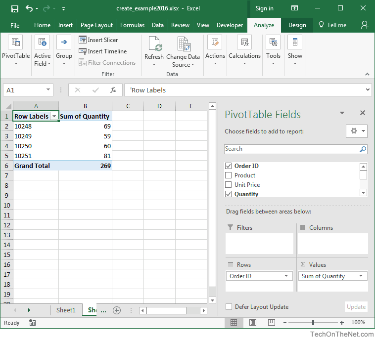
Multi-level Pivot Table in Excel (In Easy Steps) First, insert a pivot table. Next, drag the following fields to the different areas. 1. Order ID to the Rows area. 2. Amount field to the Values area. 3. Country field and Product field to the Filters area. 4. Next, select United Kingdom from the first filter drop-down and Broccoli from the second filter drop-down.
Using Pivot Tables in Excel 2016 | UniversalClass
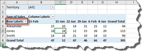
Excel Pivot Table Subtotals - Contextures Excel Tips 01.02.2022 · In the pivot table shown below, Service is in the Row Labels area, Lead Tech is in the Column Labels area, and Labor Cost is in the Values area. Because Service is the only field in the Row Labels area, it has no subtotal. Multiple Row Fields. When you add another field to the Row Labels area, a subtotal is automatically created for the first ...

Naming Columns | CLEARIFY
Pivot table row labels in separate columns - Audit Excel So when you click in the Pivot Table and click on the DESIGN tab one of the options is the Report Layout. Click on this and change it to Tabular form. Your pivot table report will now look like the bottom picture and will be easier to use in other areas of the spreadsheet and in our opinion is also easier to read.

Pivot Tables in Excel: Beginner’s Guide
Formula1, Formula2 appearing as row items in pivot table ... if you select a row item and go to the botttom right of the cell to the black cross hairs and drag down, it inserts formula1, formula2 formula3 depend how far you dragged it, and the appear in multiple cells in the pivot table. The solution is as listed above. Going to pivot table, Analyse, Fields, items & sets, solve order and deleting the ...

excel - Pivot Table shows blank value labels - Stack Overflow
Pivot Table adding "2" to value in answer set 1) Right click your pivot table -> Pivot table options -> Data -> Change "Number of items to retain per field" to NONE 2) Wipe all rows in your data source except for the headers 3) Refresh the pivot table 4) Save, and close all instances of Excel 5) Reopen the file, and paste your data 6) Refresh the pivot table
33 Pivot Table Blank Row Label - Labels Database 2020
Combining two+ Columns to form one Row label column in ... Re: Combining two+ Columns to form one Row label column in Pivot Table Select a cell in your pivot table. Press Alt, then D, then P (i.e. in succession; not all at the same time), to call up the Pivot Table Wizard. Click "" button twice.
Multiple Row Filters in Pivot Tables - YouTube
How to make row labels on same line in pivot table? Make row labels on same line with setting the layout form in pivot table As we all know, the pivot table has several layout form, the tabular form may help us to put the row labels next to each other. Please do as follows: 1. Click any cell in your pivot table, and the PivotTable Tools tab will be displayed. 2.

How to Show the Percentage of Row Total in the Pivot Table - MS Excel | Excel In Excel
How to reverse a pivot table in Excel? To reverse the pivot table, you need to open PivotTable and PivotChart Wizard dialog first and create a new pivot table in Excel. 1. Press Alt + D + P shortcut keys to open PivotTable and PivotChart Wizard dialog, then, check Multiple consolidation ranges option under Where is the data that you want to analyze section and PivotTable option under What kind of report do you …
Post a Comment for "42 excel pivot table 2 row labels"